My Computer Science Research : Maximizing Single-Commodity Unsplittable Network Flow

Hi readers! In this post, I will share my undergoing computer science research project. I haven’t finished and I am still working on it, so this report will explain all of my progress and development of the solution, including those that had failed. If you like it, please hit the like button! Any feedbacks or suggestions are also welcomed.

Maximizing Single-Commodity Unsplittable Network Flow 

Introduction

The single commodity unsplittable network flow problem is a special case of the unsplittable network flow problem. In brief, the unsplittable network flow problem is a problem involving a source and a sink where all the flows have to be sent on a single path. The single commodity unsplittable network flow problem is similar to the general version, except that only one flow has to be unsplittable. The final goal of this problem is to maximize the flows that are sent.

Until now, the unsplittable network flow problem has not been resolved completely yet. The offered solutions still solve the problem, but they usually violate some of the conditions. Inefficient time complexity also often becomes another obstacle.

In this report, the author will elaborate the rigorous definition of the problem in detail. Also, since the final solution has not been found yet, the progress and development of the solution, including those that were failed, will be fully explained. It is worth to be noted that for the sake of simplicity, the author decided to turn this problem into an analogous one: assignment of international and Korean students to their respective classes.

 

Research Background

Definition 1: A network is defined as a directed graph, denoted by G(V,E), that consists of a vertex s ∈ V and a vertex t ∈ V as the source and sink nodes, respectively. Furthermore, every directed edge from u to v, denoted by (u,v) ∈ E, has a capacity, denoted by c(u,v), and its value is positive (c(u,v)>0). Also, since the graph is directed, c(u,v) may not be equal to c(v,u) with a condition that both (u,v) ∈ E and (v,u) ∈ E.²

Definition 2: A flow in a network is described as an association of a nonnegative flow, denoted by f(u,v), to every edge (u,v) ∈ E, such that the flow is less than or equal to the capacity (f(u,v) ≤ c(u,v)) and the sum of incoming flows is equal to that of outcoming flows ( ∑_u∈V               f(u,v) = ∑_w∈V f(v,w)) for every vertex v ∈ V.²

Definition 3: The cost of the flow is defined as ∑_v f(s,v) where s is the source node.²                                                                              

Definition 4: An augmenting path is a path from the source node to the sink node (s to t) in the residual network such that every edge has a positive capacity (c(u,v)>0). The purpose of this path is to increase the flow in the original directed graph.²

Definition 5: For an edge (u,v), the residual capacity, denoted by c_f, is defined as the difference between the capacity and the flow in the original graph (c_f(u,v) = c(u,v) – f(u,v)).²

Definition 6: Bottleneck edge is an edge which has the minimum cost in a particular path.³

Definition 7: A flow in a network must be conserved. In other words, for all u ∈ V \ {s,t}, ⁵

1. Residual Graphs

A residual graph is a graph that has the same vertices as the original network of directed graph and one or two edges for each edge in the original. If the flow along the edge (u,v) is less than the capacity in the original graph, then there is a forward edge (u,v) with a residual capacity equals to the difference between its capacity and its flow in the original graph (c_f(u,v) = c(u,v) – f(u,v)). If the flow along the edge (u,v) is equal to the capacity in the original graph, then the residual capacity of the forward edge is 0 and it is not included in the residual graph. In both of those two cases, there is always a backward edge (v,u) with a residual capacity equals to the difference between its capacity and its flow in the original graph (c_f(v,u) = c(v,u) – f(v,u)). Furthermore, by using theorem 1, c_f(v,u) = c(v,u) – f(v,u) = c(v,u) + f(u,v). However, the capacity of the backward edge is 0 (c(v,u) = 0) since a backward edge does not exist in the original graph, so the residual capacity of the backward edge is equal to the flow along the edge (u,v) in the original graph (c_f(v,u) = c(v,u) + f(u,v) = 0 + f(u,v) = f(u,v)).⁴

2. Ford-Fulkerson Algorithm

The Ford-Fulkerson algorithm is a greedy algorithm that can solve the maximum flow problem. The algorithm can be outlined in 3 simple steps: initialize the value of the flow to 0, improve the current solution by using the augmenting path from the source node to sink node as long as it is available, and take the value of the flow as the answer.⁵

The algorithm can be described as the following:

1. Initialize a residual graph as the original graph
2. Initialize a variable maxflow = 0
3. While there is an augmenting path
   1. Find an augmenting path by using BFS (Breadth First Search) or DFS (Depth First Search) on the residual graph
   2. For each edge (u,v) in the augmenting path
      • Decrease the residual capacity on the edge (u,v) by the value of bottleneck edge\
      • Increase the residual capacity on the edge (v,u) by the value of bottleneck edge
   3. Increase the value of maxflow by the value of bottleneck edge
4. Return the value of maxflow⁸

Definition 7: Level graph is a graph in which levels are assigned to all nodes. In here, level of a node is defined as the shortest distance, in terms of number of edges, from the source node to a particular node.⁷

Definition 8: Blocking flow is a flow when no more flow can be sent by using the level graph. In other words, there does not exist a path from the source node to the sink node such that the vertices have ordered levels of 0, 1, 2, …⁷

3. Blocking Flow Algorithm

In this algorithm, for each vertex, a list of edges to the next level is established. Furthermore, the current edge will also be tracked. At the beginning, the pointer refers to the first edge in the list. After that, we will advance the current pointer of the nodes. There is no need to track at the edges that were already passed by the pointer. Note that in this algorithm, advance means that if the current vertex v is not the sink and there is a forward edge (v,u), then add that edge to the current path and set the current vertex to be u.

First, perform DFS to find a path from s to t. If a path cannot be found, then advance the current edge pointer and perform DFS to the next neighbor. Repeat this process until a path can be found. However, if there are no more neighbors and no path can be found, then return “no path found”. Otherwise, return “path found”.

When the top level DFS returns with “path found”, the flow is augmented along the path, and the process continues from the source again. Once the top level DFS returns with “no path found”, then a blocking flow is found.¹⁴

4. Dinic’s Algorithm

Dinic’s algorithm is another algorithm that can solve the maximum flow problem. Similar to the Ford-Fulkerson algorithm, Dinic’s algorithm also uses residual graph and BFS in a loop. However, in this algorithm, BFS is used differently. BFS is used to check if it is possible to send more flows and also to construct the level graph. In addition, DFS is also used to find the blocking flow in the level graph.¹⁴

The algorithm can be described as the following:

1. Initialize a residual graph as the original graph
2. Initialize a variable maxflow = 0
3. While there is a path from the source node to the sink node
   1. Use BFS on the residual graph to construct the level graph (assign levels to vertices) and to check if more flow is possible
   2. For each blocking flow in the level graph that is found by DFS
      • Update the residual capacity, by using the forward edge and backward edge (same procedure as in Ford-Fulkerson algorithm), in the blocking flow according to the value of bottleneck edge
      • Increase the value of maxflow by adding the value of bottleneck edge

4. Return the value of maxflow⁸

 

5. Push-Relabel Algorithm

Similar with the previous algorithms, this algorithm can also be used to solve the maximum flow problem. Push-relabel algorithm also works on residual graph. However, this algorithm works on one vertex at a time instead of finding an augmenting path by searching throughout the whole residual graph. Furthermore, unlike in the above algorithms, this algorithm allows the inflow to be greater than the outflow provided that the final flow has not been reached yet. As indicated by its name, this algorithm uses the push() and relabel() function.⁹

Definition 9: Preflow is similar to flow: it follows the flow conservation and also the capacity rule. However, pre-flow is defined as a non-deficient flow, which means that the net flow entering a node, except the source, is non-negative.¹²

Definition 10: Excess flow is defined by e(u) = . A vertex u ∈ V \ {s,t} is active or overflowing if e(u) > 0.¹⁰

Definition 11: Height is a function defined as h: V à N. It has three properties: h(s) = |V|, h(t) = 0, and h(u) ≤ h(v)+1 for every residual edge (u,v).¹⁰

There are three basic operations in Push-Relabel Algorithm¹¹:

1. Initialization

The first step in this operation is to form the residual graph from the given graph. After that, set excess flow values of every vertex, except the source and sink, as 0 and height of every vertex, except the source, as 0. For the source vertex, set its height to the total of number of vertices in the graph (h(s) = |V|). Then, initialize the flow of every edge as 0. After that, perform an initial push to all vertices adjacent to the source vertex with an amount equal to the respective capacity. As a result, the excess flow of vertices adjacent to the source vertex is equal to the respective capacity.

2. Push

This operation is used to push the flow from active or overflowing vertices to their adjacent vetices with smaller height in residual graph. The amount of pushed flow is equal to min {e(u) , c_f(u,v)}.

3. Relabel

This operation is used when a vertex is active or overflowing and there are not any of its adjacent vertices having smaller height. In this case, the height of that vertex is relabeled or increased by minimum of adjacent height in the residual graph + 1.

Note that whenever a push of flow is performed from vertex u to v, the residual graph has to be updated by using forward and backward edge with the same procedure as in Ford-Fulkerson algorithm.

With these three basic operations in mind, the generic algorithm can be described as follows⁹:

• Initialize
• While there is an applicable Push or Relabel operation, execute the operation
• Return the maximum flow

6. Correctness Proof of Ford-Fulkerson Algorithm¹

Definition 12: A cut (S,T) of flow network G(V,E) is a partition of V into S and T = V \ S (a set of all the vertices except the source) provided that s ∈ S and t ∈ T.

Definition 13: The net flow f(S,T) across the cut (S,T) is defined as f(S,T) =  – .

Definition 14: The capacity of the cut (S,T) is defined as c(S,T) =

Definition 15:

Lemma 1: Let f be a flow in a flow network G with source s and sink t, and let (S,T) be any cut of G. Then, the net flow across (S,T) is f(S,T) = |f|.

Proof: From definition 7, From definition 15, , S  T = V and S  T = , |f| =

Corollary 1: The value of any flow f in a flow network G is bounded from above by the capacity of any cut of G. In other words, |f| ≤ c(S,T).

Proof: By using lemma 1 and definition 14. |f| = f(S,T) =   .

Theorem 1 (Max-flow min-cut theorem): If f is a flow in a flow network G = (V,E) with source s and sink t. Then, the following conditions are equivalent:

1. f is a maximum flow in G.
2. The residual network G_f does not contain any augmenting paths.
3. |f| = c(S,T) for some cut (S,T) of G.

Proof: Suppose that there is an augmenting path in residual network G_f. Then, f could be increased, which means f is not a maximum flow in G. Hence, by contraposition, a) à b). Now, suppose that b) is true. Let’s define S as a set of vertices v  V such that there exists a path from s to v in G_f. and T = V \ S. Then, by definition 12, the partition (S,T) is a cut. Also, consider a pair of vertices  and f (u,v)  f(u,v) = c(u,v) because otherwise, (u,v) _f (a set of edges in residual graph), which means that v belongs to set S. If (v,u) since otherwise, c_f(v,u) = f(u,v) > 0 and (u,v) _f, which means that v belongs to set S. Hence, by using definition 13, f(S,T) =  –  We can conclude that b) à c). By corollary 1, c) à a)

As a consequence, the Ford-Fulkerson algorithm is correct because when it is completed, the residual network G_f does not contain any augmenting paths, which by theorem 1, means that the flow in G is the maximum one.

7. Time Complexity of Ford-Fulkerson Algorithm¹

The Ford-Fulkerson algorithm might fail to terminate only if the edge capacities are irrational numbers. Hence, let’s assume that the capacities are rational numbers. In this case, appropriate scaling transformation can applied to change all the capacities into integral numbers. Now, let f* be a maximum flow in the transformed network. Then, the while loop will be executed at most |f*| times since the flow value increases by at least 1 in each iteration, with the upper bound f*. By using either BFS or DFS, finding augmenting path inside the while loop takes O(V+E’) = O(E), where E’ is the set of edges in G_f. Hence, the total running time is O(E|f*|).

8. Correctness Proof of Push-Relabel Algorithm¹

Lemma 2: During the execution of Push-Relabel algorithm on G(V,E), for each vertex u h(u) never decreases. Furthermore, a relabel operation that is applied to a vertex u increases h(u) by at least 1.

Proof: Suppose that we want to relabel a vertex u. Then, for all vertices v that satisfies (u,v)  E_f, h(u) ≤ h(v). Hence, h(u) < (minimum of all h(v) provided that (u,v)  E_f,) + 1. As a consequence, the operation must increase h(u).

Lemma 3: The execution of Push-Relabel algorithm on G(V,E) maintains h as a height function.

Lemma 4: There is no path from s to t in G_f.

Proof: Suppose that G_f  contains some paths from s to t. Let the shortest one be p = (v₀, v₁,…, v_k) where v₀ = s, v_k = t, k < |V| (assume that p is a simple path). Also, for i = 0, 1, …, k-1, (v_i,v_i+1)  E_f, |V| = h(v0) ≤ h(v₁) + 1 ≤ h(v₂) + 2 ≤ …. ≤ h(v_k) + k = k, which is a contradiction. Hence, G_f  cannot have any paths from s to t.

Lemma 5: An overflowing vertex can be either pushed or relabeled.

Proof: Let u be an overflowing vertex. For any (u,v)  E_f , h(u) ≤ h(v) + 1. If h(u) = h(v) + 1, then the push operation can be applied on vertex u. If a push operation cannot be applied on vertex u, then for all (u,v)  E_f, h(u) < h(v) + 1  <=>  h(u) ≤ h(v). Hence, a relabel operation can be applied on vertex u.

Definition 16: Loop invariant is defined as property of a program loop that is true before and after each iteration.

The correctness of generic push-relabel algorithm can be proved as below:

• Loop invariant: f is a preflow whenever the while loop is executed¹⁵
• Initialization: f is a preflow
• Maintenance: We know that there are only push and relabel operations inside the while loop. If f is a preflow before the push operation, it will remain as a preflow afterward. On the other hand, relabel operation only affects the height attributes and not the flow values. Hence, relabel operation does not affect whether or not f is a preflow.
• Termination: By Lemma 5 and the loop invariant, each vertex in V, except the source and sink, is not overflowing. Hence, f is a flow. By lemma 3, h is still a height function at termination. Also, by lemma 4, there is no path from s to t in G_f. Hence, by theorem 1, f is a maximum flow.

9. Time Complexity of Push-Relabel Algorithm¹

Lemma 6: For any overflowing vertex x, there is a simple path from x to s in G_f..

Lemma 7: At any time during the execution of Push-Relabel algorithm on G, h(u) ≤ 2|V| – 1 for all u

Proof: Since the source s and the sink t will never be overflowing (by the definition), their height will never change. Hence, h(s) = |V| ≤ 2|V| -1 and h(t) = 0 ≤ 2|V| – 1. In the case of any vertex u After relabeling, the vertex u becomes overflowing. By lemma 6, there exist a simple path from u to s in G_f. Let such a simple path be p = (v₀, v₁,…, v_k) ) where v₀ = s, v_k = t, k ≤ |V| – 1. Also, for i = 0, 1, …, k-1, (v_i,v_i+1)  E_f. Hence, by lemma 3, the height function is maintained after the operation, so h(v_i)  h(v_i+1) + 1. Hence, h(u) = h(v₀) h(v_k) + k  h(s) + |V| – 1 = |V| + |V| – 1 = 2|V| – 1.

Corollary 2: During the execution of of Push-Relabel algorithm on G, the number of relabel operations is at most 2|V| – 1 per vertex and at most (2|V| – 1)(|V| – 2) < 2|V|² overall.

Proof: Since we can’t apply relabel operations on the source s and the sink t, there are only |V| – 2 vertices that can be relabeled. Let u . By lemma 7, the relabel operation increases h(u) from 0 to at most 2|V| – 1. Hence, u is relabeled at most 2|V| -1 times. As a conclusion, the total number of relabel operations is at most (2|V| – 1)(|V| – 2) < 2|V|².

Definition 17: A saturating push is a push when edge (u,v) in G_f becomes saturated. In other words, c_f(u,v) = 0 afterward.

Lemma 8: During the execution of Push-Relabel algorithm on G, the number of saturating pushes is less than 2|V||E|

Proof: For any pair of vertices u,v , saturating pushes from u to v and from v to u are counted together, calling them the saturating pushes between u and v. We know that if there are any such pushes, at least either (u,v) or (v,u) Suppose that there is a saturating push from u to v. This means h(u) = h(v) + 1. If we want another push from u to v to happen, there must be a push from v to u first since the forward edge from u to v already disappeared after the initial saturating push. For this to happen, h(v) = h(u) + 1 must be satisfied. By lemma 2, h(u) never decreases, so to achieve h(v) = h(u) + 1, h(v) must increase by at least 2 (h(u) = h(v) + 1 ßà h(v) = h(u) – 1 ßà h(v) + 2 = h(u) – 1 + 2 = h(u) + 1). Similarly, h(u) must increase by at least 2 between saturating pushes from v to u. By lemma 7, we know that height starts from 0 to a maximum of 2|V| (h(u) ≤ 2|V| – 1 ßà h(u) < 2|V|). This means that the number of times any vertex can have its height increase by 2 is less than |V|. Since at least one of h(u) and h(v) must increase by 2 between any two saturating pushes between u and v, there are fewer than 2|V| saturating pushes between u and v. Hence, the total number of saturating pushes is less than 2|V||E|.

Definition 18: A potential function is defined as  =

Lemma 9: During the execution of Push-Relabel algorithm on G, the number of non-saturating pushes is less than 4|V|²(|V| + |E|)

Proof: Initially,  = 0. After a relabel operation is applied on vertex u,  increases by less than 2|V| since the set over which the sum is taken is the same and by lemma 7, h(u) ≤ 2|V| – 1. Furthermore, a saturating push from u to v increases  by less than 2|V| since no heights change and only vertex v, in which by lemma 7, h(v) ≤ 2|V| – 1, can be overflowing. On the other hand, a non-saturating push from vertex u to v decreases by at least 1. Before the non-saturating push, u was overflowing while v may or may not be overflowing. After the push operation is applied on u, it cannot be overflowing anymore because the amount of flow pushed from u to v is the same with e(u) and e(u) is reduced by this amount to 0. Moreover, if v is not the source, it may or may not be overflowing after the push. Hence,  is decreased by h(u) and is then increased by either 0 or h(v). h(u) = h(v) + 1 <=> h(v) – h(u) = 1, so overall, is decreased by at least 1. By corollary 2 and lemma 8, the increase in  is limited to be less than (2|V|)(2|V|²) + (2|V|)(2|V||E|) = 4|V|²(|V| + |E|). Since   0, the total amount of decrease, which means the total number of non-saturating pushes, is less than 4|V|²(|V| + |E|).

Putting together corollary 2, lemma 8, and lemma 9, it can be concluded that during the execution of Push-Relabel algorithm on G, the number of basic operation is O(V²E).

10. Analysis of Blocking Flow Algorithm¹⁴

Claim: The algorithm can always find a blocking flow.

Proof: Let’s assume that the edges passed by the pointer are indeed useless. Notice that we can only say that an edge (u,v) is useless when DFS(v) returns with “no path found”, that is when all of edges (v,w) are also useless. When path augmentation occurs, it will only remove forward edges from a particular level to the next level and add the backward edge. Hence, when the current edge pointer is advanced, then that edge is useless.

Claim: The time complexity of the algorithm is O(nm), where n is the number of vertices and m is the number of edges in G.

Proof: There are only two possibilities for DFS: returns with “path found” or “no path found”. In the case where DFS returns with “no path found”, since there are m edges then there are at most m calls. In the case where DFS returns with “path found”, the calls come in groups of l where l is the number of levels in the level graph. Every l of them will cause an edge to become saturated. Hence, the total number of such calls is at most lm ≤ nm.

Introduction (Transformation From Single Source Multicommodity Flow Problem to Single Source Unsplittable Flow Problem)¹⁶

Given a directed graph G(V,E) with a  single source s and multiple terminals t1,t2,…, tk with corresponding demands d1,d2,…,dk, each having value greater than 0. Each terminal is located at a node in the graph and multiple terminals can occupy the same node. A flow meets the demands di if the net inflow at every node, except the source, is equal to sum of the demands of terminals at that node.

The single source multicommodity flow problem happens when we want to find whether there is a flow that can meet all the demands while not exceeding capacities that are assigned to the edges. The solution to this problem is a flow such that f: E –> [0,∞) on the graph. Notice that this solution only tells the total amount of flow at a particular edge, without telling the amount of individual flow for each commodity.

To give more information, the solution can be modified into flow with allocations. This is a flow that solves multicommodity flow problem together with a decomposition f = f1 + f2 + … + fk of f into one flow for each commodity. The flow fi must have an outflow di at s, and an inflow di at t.

Fortunately, if we can already find a flow to solve the problem, we can find the allocations for that flow. First, decompose the flow into paths and cycles. Then, remove all the cycles. There is no issue at this step since the resulting flow still satisfies the demands. Finally, assign edges from s to each ti to meet the demand di.

A flow with allocations f = f1 + f2 + … + fk is unsplittable if for each i there exists a path from s to ti such that fi is 0 everywhere except on that path.

Let’s call arbitrary flows that are not necessarily unsplittable as fractional flows.

Theorem 1: Given a fractional flow f meeting demands di. Then, there exists an unsplittable flow meeting the same demands such that the total flow on any edge e is at most f(e) + dmax where dmax is the largest demand.

Proof of Theorem 1

The proof is an algorithm that takes an initial fractional flow and produces desired unsplittable flow.

1. Movement of Terminals

In this step, the goal is to move the terminals closer to the source to reduce the problem into smaller sub-problem. Let there be terminal ti at vertex v. Suppose that after executing the algorithm, the unsplittable path for ti uses edge (u,v). Then, terminal ti is moved from v to u and the flow on edge (u,v) is decreased by di units (the amount of demand by that terminal). If we can solve this, then we just need to add di units back to edge (u,v) to get the final solution. This step stops when the all terminals are at source s.

2. Alternating Cycles

The cycles are constructed by these steps:

1. Start at any vertex v
2. Never go back on the same edge that you have just arrived on
3. Follow a forward edge whenever possible
4. Follow a backward edge if it is not possible to follow a forward edge without violating step 2
5. Stop when meeting a vertex w that is already visited previously. The resulting closed loop (without the path from v to w) is an alternating cycle.

After an alternating cycle is found, we can augment flow along it. We need to simultaneously decrease the flow on forward edge and increase the flow on the backward edge by the same amount until one of the following happens:

• The flow on some forward edges reaches 0
• For some terminal ti at some vertex u and for some backward incoming edge (v,u), f(u,v) (flow on edge (u,v)) increases (from below di) to di

If the first case happens, then the edge is removed from the graph.

3. The Complete Algorithm

Definition 1: An edge (u,v) is singular if v and all the vertices reachable from v have out-degree at most 1. Equivalently, the vertices reachable from v induce a directed path.

Using this definition, we can make sure that the flow on each edge does not increase by more than dmax. This is done by ensuring that at most 1 terminal moves across e after it becomes singular. We can do this by making sure that whenever a terminal moves across a singular edge, the singular edge is left with zero flow and is removed from the graph.

The rules for moving terminals at each iteration of the algorithm: move terminal ti from v to u whenever either

1. (u, v) is a singular edge and f(u, v) = di , or
2. (u, v) is not singular and f(u, v) ≥ d

If both are possible, then we need chose a) instead of b).

The second issue is to ensure that we can always find an alternating cycle. We know that the algorithm can fail to find an alternating cycle if and only if it arrives at a degree-1 (including both incoming and outgoing edges) vertex via its only incident edge. Fortunately, it can be proven that this case would never happen.

Case 1: Vertex with a single outgoing edge and no incoming edges.
We know that this vertex must be a source (due to the flow conservation). If the algorithm starts at the source when building an alternating cycle, then it can just move forward along the single outgoing edge. Since backward edges are singular, the only way for a backward path goes to the source is if the single outgoing edge from the source is singular. If this happens, then all terminals should have already been moved to the source.

Case 2: Vertex v with a single incoming edge (u,v) and no outgoing edges.
By flow conservation, this vertex must at least contain one terminal ti. Since (u,v) is the only incoming edge for v, f(u,v) ≥ di.

Definition 2: A terminal ti at vertex v is irregular if it has an incoming edge (u, v) with f(u, v) ≥ di. Otherwise it is called regular.

By this definition, v is an irregular terminal.

Lemma 1: A vertex containing an irregular terminal must have at least 2 incoming edges.
(Proof cannot be summarized)

This lemma contradicts the assumption that v has a single edge, so the second issue is now resolved.

Algorithm 1. (Dinitz, Garg, Goemans)
Input: G = (V, E) with source s and terminals t1, . . . , tk, demands d1, . . . , dk, fractional flow f
1. Use flow decomposition to make f acyclic.
2. Move terminals closer to the source wherever possible.
3. Identify singular edges and label them as singular.
4. Find an alternating cycle and augment flow along it.
5. Move terminals according to rules (1) and (2) above, using the labels from step 3.
6. If all terminals have reached the source, stop. Otherwise go to step 3.

Unsplittable Flow Problem¹⁷

Input:

1. Directed graph G(V,A). A in here refers to arcs, which are directed edges.
2. Integer capacity u_ij ≥ 0 for every (i,j)
3. Specified source-sink demand pairs in V, s_1-t_1,…,s_k-t_k.
4. Integer non-negative demands d_1,…,d_k each corresponding to the respective source-sink pair.

Goal: For each s_a-t_a (a=1,…,k), find an s_a-t_a path P_a, such that for every (i,j)  A, . In other words, we need to send demand of each source-sink pair on a single path such that it doesn’t exceed the capacities on all arcs.

One of the optimization variants of the problem is where s_a = s for all a = 1, 2, …, k and in addition there is a cost c_ij ≥ 0 for each arc (i,j)  A. The goal is defined as above, but with an objective of minimizing the cost.

Decision Version

The goal is to answer whether there exists an unsplittable flow of cost ≤ B.

Observation: The splittable flow problem is solvable in polynomial time and the optimal solution has integrality property.

Procedure: First, we can try to find an optimal splittable flow. Suppose that the optimal splittable flow has cost ≤ B. We want to find an approximated unsplittable flow. Here the notion of approximation can refer to two aspects:

1. Minimum congestion: Finding an unsplittable flow, where the capacity constraint of each arc (i,j) is not violated by more than a factor of α (α>1). We want to minimize α.
2. Minimum number of routing rounds: Sending the flow in rounds, where in each round we respect the capacities of all arcs. We want to minimize the number of rounds.

An Algorithm

Assume that max_a d_a ≤ min_(i,j)A u_ij.

Theorem: Assume there exists a splittable flow of cost ≤ B. Then in poly-time one can find an unsplittable flow such that one of the following holds:

1. The flow over any arc (i, j) ∈ A is ≤ 3u_ij.
2. The flow can be sent in at most 8 rounds.

Key idea of the theorem:

1. Increase capacities
2. Re-route the splittable flows, which have integraliry property.
3. If d_a = d and all capacities are multiples of d, the unsplittable flow problem is reduced to min-cost flow problem.

Algorithm for a special case: Let d_min = min_a d_a, d_max = max_a d_a and u_min = min_(i,j)∈A u_ij. Assume that for each a =1,..,k, d_a = d_min 2^q for some q ∈ N.

 

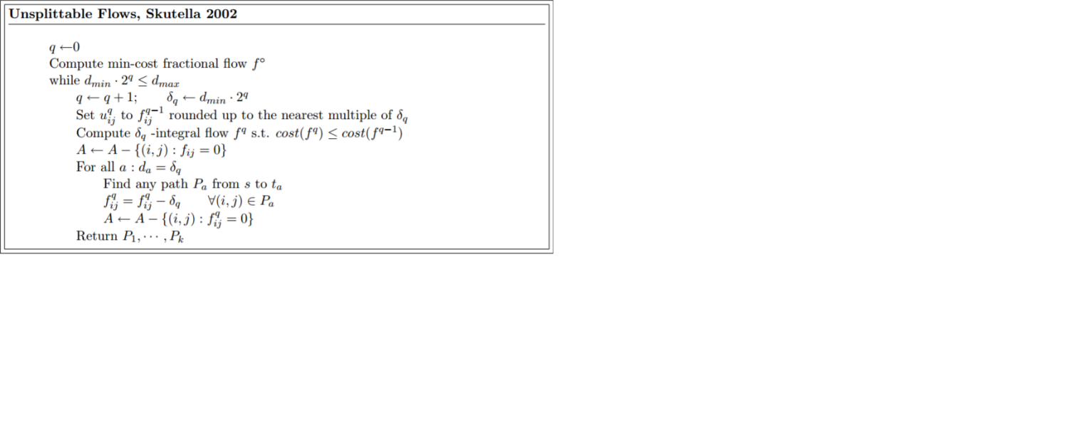
In each iteration,  is the new unit of measure. Also, in each iteration k, the previous flow f^k-1 is still important.

Single source case: there is one source node s and k sink nodes t1,…,tk with respective demands d1,…,dk.

If there is no fractional flow, there can’t be an unsplittable flow.

Theorem: Assume fractional flow exists, and that d_max ≤ u_min. Then we can find an unsplittable flow of cost no more than the fractional flow using capacity 3u_ij, ∀ (i, j) ∈ A

Theorem: The algorithm finds an unsplittable flow using capacity uij + dmax of cost no more than the fractional flow f₀.

Corollary: For any (i,j), the sum of all demands but one using arc(i, j) is bounded by f⁰_ij − d_min.

General case:

1. Round demands up to have the form d_min2^q . Thus, no demand increases by more than a factor of 2. In this case, the capacity needed on each edge is bounded by 3uij . However, the costs might increase by a factor of 2.
2. Round demands down to have the form d_min2^q. Suppose d’a = (da rounded down).

 

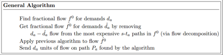
Theorem: The above algorithm returns an unsplittable flow of cost no more than the fractional flow using capacity ≤ 3u_ij.

 

Research Result

Special Case of Unsplittable Flow Problem

Let’s formulate this as a problem of allocating both of international students and domestic students on each course with a condition that all of the international students have to be allocated at the same class.

Simple Case (Complete Bipartite Graph)

Let there be m international students and n domestic students who apply to a course A. There are k classes for this course and each class has a maximum capacity of c. Maximize the number of students that can be allocated.

Solution:

1. If c < m, since we have to put m students at the same class, we cannot allocate any international students. In this case, the rest of n domestic students can be exhaustively allocated and the worst case happens when there is leftover of n-c*k unallocated students.
2. If cm, then we can put the all m international students in 1 class and fill the rest of m-c spots with n domestic students. In this case, if k , then we can assign the rest of n-(m-c) domestic students exhaustively to the remaining k-1 classes with the worst case being n-(m-c) – c*(k-1) unallocated domestic students.

The international students must be prioritized over the domestic students because the domestic students can still be distributed to other classes if one class already reaches its maximum capacity. However, for international students, if we cannot find a class which can fit all of them, then we can’t allocate all of them. In other words, we will “lose” all of them.

General Case (Complete Bipartite Graph)

Let there be m₁, m₂, m₃, …, m_i international students who apply to courses A₁, A₂, A₃,  …, A_i respectively. Let there be n₁, n₂, n₃, …, n_i domestic students who apply to courses A₁, A₂, A₃,  …, A_i respectively. There are x₁, x₂, x₃, …, x_i classes with capacity c₁, c₂, c₃, …, c_i for each course A₁, A₂, A₃,  …, A_i.

Solution: For each course, apply the previous solution.

General Case

Let there be m₁, m₂, m₃, …, m_i international students who apply to courses A₁, A₂, A₃,  …, A_i respectively. Let there be n₁, n₂, n₃, …, n_i domestic students who apply to courses A₁, A₂, A₃,  …, A_i respectively. There are x₁, x₂, x₃, …, x_i classes with capacity c₁, c₂, c₃, …, c_i for each course A₁, A₂, A₃,  …, A_i. However, in this case, a student may not be able to be assigned to certain classes. For example, if there are two classes x₁, and x₂ for a course A₁, there might be a case such that a student can only be assigned to x₁, but not x₂.

Basic assumption: For each course, there is at least 1 class in which all of the international students can be assigned to. Also, clearly the capacity of that class must be at least equal to the number of all international students.

Observation 1: Prioritizing and exhausting the domestic students is not beneficial at all. Consider an example where there is no more domestic students available while there are still some empty spots in a particular class. If the number of international students is less than the number of empty spots, then we cannot assign any of them and we end up leaving the empty spots.

Observation 2: From observation 1, this means prioritizing the international students will probably be a good strategy. This is because the domestic students can be splitted and assigned individually (if they are able to be assigned!) to fill the empty spots while we cannot always do that to international students since they have to be assigned all together at one particular class.

Observation 3: However, blindly or randomly putting all international students in a particular class is also not a good idea. Consider the case when there are two classes x₁ and x₂ while all the domestic students can only be assigned to x₁ (but not x₂) and the international students can be assigned to both of the classes. If we assign all the international students to x₁ such that the maximum capacity is reached, none of the domestic students can be assigned and so class x₂ is empty. On the other hand, if we assign all the international students to x₂, then we can assign as many domestic students as possible to x₁.

Solution: For each course, find and list out common classes in which all the international students can be assigned. Among those classes, select the class which has the least number of potential domestic students that can be assigned with a condition that the capacity of that class must be at least equal to the number of international students and assign all of the international students. After that, put as many as possible domestic students in the classes in which they can be assigned to.

Flaw: If the number of international students is 0, then the above method should have solved the max flow problem. However, it doesn’t. Hence, we need to change the way we assign Korean students

Updated solution:

1. For each domestic student, make an array to count how many possible classes that they can be assigned to.
2. Sort the array from the smallest to the largest to determine the order of assignment.
3. Assign exhaustively. For students who only have one choice, just assign them to that class until the max capacity is reached. For students who have more than one choice, it doesn’t matter which class they are assigned to (if a student has choice A and B, it doesn’t matter whether he is assigned to A or B). However, when there is no spot left, assign the student to the next choice of class.

Flaw: Still incorrect. The solution actually should contain maximum flow algorithm so that at least it can solve the special case where there are no international students.

Updated problem statement: Given two sources s₁ and s₂ where s₁ is international students and s₂ is domestic students. Let there be ti classes (terminals) each with capacity ci. The assignment for international students cannot be separated (either assign all of them to the same class or don’t assign any of them). In addition, the number of students in a particular class cannot exceed its capacity. The goal of this problem is to maximize the number of assigned students.

Second update of problem statement: Given a source and a sink. Also, there are nodes in between: one node for international students (combined), and several nodes for Korean students (separated). There are also classes (terminals) which have their own maximum capacities. In this problem, the international students have to be assigned together to the same class (unsplittable). It is not necessary to assign all the international students.

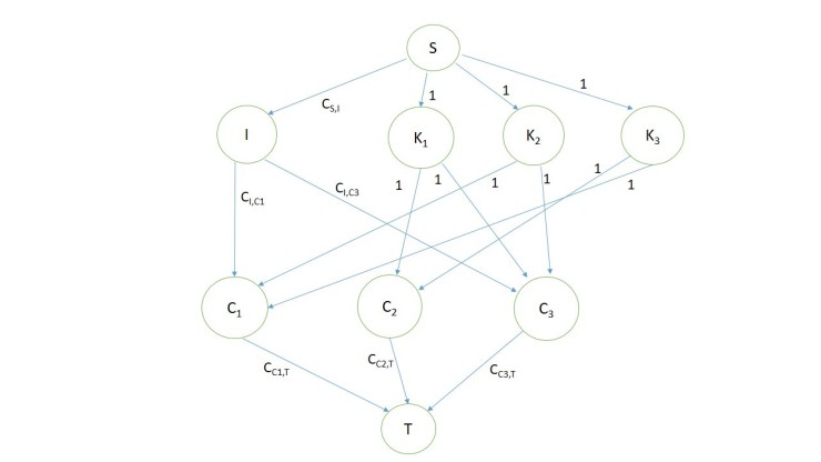
Third update of problem statement: Given a directed graph G(V,E). The graph consists of one node for international students, denoted as I, and x other nodes, labelled as k₁, k₂, …, k_x, for Korean students. There are nodes of y classes, labelled as c₁, c₂, …, c_y. Two special nodes, which are source s and sink t (s, are also given. Hence, the set V is defined as V = { I, k₁, k₂, …, k_x, c₁, c₂, …, c_y, s, t }. There are edges from the source s to I, k₁, k₂,…, k_x. There exist edge (s, I). The capacities of edges from s to I denote the number of international students. Also, there is edge (s, k_i), in which the capacity denotes that there is one Korean student called k_i. If there is at least one student from I who can be assigned to c_j, there has to be an edge (I, c_j) between them. The capacity of edge (I, c_j) denotes the number of international students who are available for the class c_j. If a Korean student k_i can be assigned to c_j, there must be an edge (k_i, c_j). The capacity of edge (k_i, c_j) means that a Korean student k_i is available for the class c_j. Finally, there must be edges (c,t_j), in which the capacities denote the maximum number of students who can occupy the class t_j. In this problem, the international students have to be assigned together to the same class (unsplittable). Furthermore, it is not necessary to assign all the international students. The final goal is to maximize the number of assigned students.

 

Solution:

Using the idea of prioritizing international over domestic students:

1. List all of availability of each international student
2. For each class, count how many potential students can be assigned
3. Sort the classes from the one that has the largest number of potential students to the smallest number of potential students
4. Executing from the class which has the maximum number of potential students, compare the capacity and the number of potential students. If the capacity is at least as large as the number of potential students, then assign all those students. Otherwise, go to the next largest class and repeat this procedure
5. Assign the domestic students by using one of the described maximum flow algorithm

Flaw: Let there be 20 international students in total. Suppose that there are 10 international students that are available for the first class, 18 international students that are available for the second class, and 14 international students that are available for the third class. Let there be 10 domestic students and suppose that all of them can only be assigned to the second class. Let the capacity of the first class to be 12, second class to be 15, and third class to be 21. Using the above algorithm, all international students will be assigned to the second class, but since the capacity is only 15, there will be 5 international students that are left. Hence, there will be a total of 15 unassigned students (international and domestic altogether). The number of unassigned students could actually be minimized further by assigning all the international students to the third class             and the domestic students to the second class. This time, there are only a total of 6 unassigned students.

Updated solution:

1. Assign the international students together to any one of the classes.
2. Apply one of the maximum flow algorithms that is described above.
3. Make an array that stores how many Korean students who cannot be assigned and another array that stores the data of students in each class.
4. Link the two arrays together.
5. Repeat step 1 and 2 to all of the remaining classes.
6. Sort the first array (that stores the number of unassigned Korean students) from the smallest to the largest
7. Use the solution of assignment that is produced by the minimum number of Korean students who cannot be assigned.

Hypothesis: The above solution can be made more efficient by assigning international students to the class which has the least forward edge from the domestic students. If there are multiple such classes, then choose the one which can accommodate more international students.

 

References

1. Introduction to Algorithm, Third Edition
2. https://lucatrevisan.wordpress.com/2011/02/04/cs261-lecture-9-maximum-flow/
3. https://www.cs.cmu.edu/~ckingsf/bioinfo-lectures/netflow.pdf
4. https://brilliant.org/wiki/ford-fulkerson-algorithm/
5. https://www.topcoder.com/community/data-science/data-science-tutorials/maximum-flow-section-1/
6. https://www.geeksforgeeks.org/ford-fulkerson-algorithm-for-maximum-flow-problem/
7. https://www.geeksforgeeks.org/dinics-algorithm-maximum-flow/
8. https://visualgo.net/en/maxflow
9. https://www.geeksforgeeks.org/push-relabel-algorithm-set-1-introduction-and-illustration/
10. https://www.topcoder.com/community/data-science/data-science-tutorials/push-relabel-approach-to-the-maximum-flow-problem/
11. https://en.wikipedia.org/wiki/Push%E2%80%93relabel_maximum_flow_algorithm
12. https://en.wikipedia.org/wiki/Flow_network#Flows
13. https://cseweb.ucsd.edu/classes/sp11/cse202-a/lecture13-final.pdf
14. http://www.cs.cmu.edu/afs/cs.cmu.edu/academic/class/15451-f14/www/lectures/lec11/dinic.pdf
15. https://en.wikipedia.org/wiki/Loop_invariant
16. https://pdfs.semanticscholar.org/379b/a072d6da4fb881a43bde55f23cd1244d3219.pdf
17. https://people.orie.cornell.edu/dpw/techreports/cornell-flow.pdf